Introduction to preprocess - package tutorial • preprocess

# packages
library(dplyr)
library(ggplot2)
library(tidyr)
library(stringr)
library(readr)
library(tibble)
library(preprocess)

Introduction

This vignette demonstrates the use of simulated datasets to illustrate the application of the fill_in and standardise functions for preprocessing environmental exposure data.

⚠️ Important: The fill_in function assumes that the variable to impute is normally distributed. It is the user’s responsibility to apply the appropriate transformation (e.g., log-transformation) to ensure normality prior to using this function. The same transformation must be applied to the Limit of Detection (LOD) to ensure consistency.

Specifically, it covers how to:

Handle values below the Limit of Detection (LOD) using the method proposed by Helsel (1990). This approach accommodates one or multiple exposure components, each with potentially different LODs.
Standardize exposure data by adjusting for protocol variables selected from a list of candidates, while also accounting for additional covariates, following the method of Mortamais et al. (2012).

The Simulated Data

The datasets used in this example were designed to resemble real-world environmental exposure data. They simulate common scenarios where LOD handling and standardization are necessary.

# load simulated data 
data("dt_exp")
data("dt_lod")

The example data (dt_exp) consists of the following variables:

4 lognormally distributed exposures exp1, exp2, exp3 and exp4, left censored (LOD), with missing data. Data below LOD is reported as “<LOD”.
batch, batch effect which is TRUE for exp1 and exp4
prot1 continuous protocol variable associated with exp2
prot2 continuous protocol variable associated with none of the exposures
season, season effect which is TRUE for exp4, in addition to the batch effect
cov1, additional covariate to be included in standardisation models

Examples of candidate protocol variables include: sample transportation time, sample defreeze time prior to measurement. Examples of additional covariates to be included in the standardisation model include: age or breastfeeding duration.

The data is in a wide format (one column per exposure), which is the usual format such data is provided by analytical laboratories.

head(dt_exp)
#>     id batch             exp1             exp2              exp3       prot1
#> 1  id8     1 1.22925099690535 2.88779888466437              <LOD -0.00954975
#> 2 id14     1 4.17231182471364  3.9394983990565              <LOD -0.38237917
#> 3 id16     1 3.55763803500625 1.75607103905869 0.561280432909913 -0.59325353
#> 4 id17     1 2.25789439366093             <LOD              <LOD -0.19531902
#> 5 id22     1 6.92484889235359 1.46692222224359 0.853212096159328 -0.06349861
#> 6 id25     1 4.96218477666339 1.39213028969762              <LOD  0.36055996
#>      prot2 season             exp4         cov1
#> 1 31.35448 Autumn 3.22925099690535 -0.122238985
#> 2 47.39001 Summer 3.17231182471364 -0.042519367
#> 3 43.81518 Summer 2.55763803500625  0.005900652
#> 4 41.45147 Spring 5.25789439366093  0.330839677
#> 5 68.25540 Spring 9.92484889235359  0.034422787
#> 6 43.87650 Summer 3.96218477666339  0.241904949

head(dt_lod)
#>    exp lod
#> 1 exp1 1.1
#> 2 exp2 1.1
#> 3 exp3 0.4
#> 4 exp4 1.7

Prepare data

Data first needs to be converted to tidy format (one row per id and per compound, one column per variable) and LOD needs to be added in new column:

# convert exposure to long format and add lod
dt_exp_long <- dt_exp |>
  pivot_longer(
    cols = starts_with("exp"),
    values_to = "val",
    names_to = "exp"
  ) |>
  left_join(dt_lod, by = "exp") |>
  mutate(
    val_num = ifelse(val == "<LOD", lod / 2, as.numeric(val))
  )

head(dt_exp_long)
#> # A tibble: 6 × 10
#>   id    batch    prot1 prot2 season    cov1 exp   val                lod val_num
#>   <chr> <int>    <dbl> <dbl> <chr>    <dbl> <chr> <chr>            <dbl>   <dbl>
#> 1 id8       1 -0.00955  31.4 Autumn -0.122  exp1  1.22925099690535   1.1    1.23
#> 2 id8       1 -0.00955  31.4 Autumn -0.122  exp2  2.88779888466437   1.1    2.89
#> 3 id8       1 -0.00955  31.4 Autumn -0.122  exp3  <LOD               0.4    0.2 
#> 4 id8       1 -0.00955  31.4 Autumn -0.122  exp4  3.22925099690535   1.7    3.23
#> 5 id14      1 -0.382    47.4 Summer -0.0425 exp1  4.17231182471364   1.1    4.17
#> 6 id14      1 -0.382    47.4 Summer -0.0425 exp2  3.9394983990565    1.1    3.94

Data description

It is important to describe data prior to pre-processing.

Detection rates and basic statistics:

Description of raw exposure data
Exposure	% < LOD	p5	Median	p95
exp1	5%	<LOD	3.55	7.39
exp2	15%	<LOD	2	4.58
exp3	31%	<LOD	0.5	1.16
exp4	5%	1.74	5.44	9.73

Exposure level distribution:

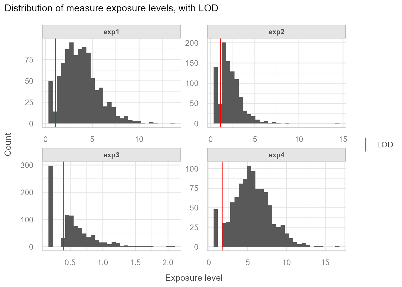
=> We observe different rates of data below LOD. Based on this, exposures that are considered having too high rates of data < LOD need to be excluded from the imputation-standardisation process. In this example exp3 will be removed from any further processing and will be categorised.

Step 1: Fill in data below LOD

The fill_in function is written to be used on tidy data (one row per id and per exposure). It is important to specify the .by argument of the mutate call in order to separately impute data below LOD for each group. This is important because this step requires computing exposure specific distribution parameters, and LOD can also vary from one exposure to another. In this simple example the only grouping variable is the exposure, but there could be more groups on which we would like to apply the fill-in procedure separately like exposure and sample period, in which case the .by argument of the mutate call would be modified to .by = c(exp, period).

Important: The fill_in function uses the method of Helsel (1990), which assumes that the variable to be imputed follows a normal distribution. In environmental epidemiology, exposure variables are often log-normally distributed. Therefore, the user must apply a log-transformation (or another appropriate transformation) to the variable before calling fill_in, and must apply the same transformation to the LOD.

The function does not perform any transformation by itself and relies on the user to ensure distributional assumptions are met.

Fill in is done like this:

# Impute data below LOD 
set.seed(113)
dt_imp <- dt_exp_long |>
  filter(exp != "exp3") |>
  mutate(
    log10_val_i = fill_in(
      var_to_fill = log10(val_num), # variable to be filled in, needs to be normal
      lod = log10(lod)              # variable containing LOD, needs to be same unit as variable to fill
    ),
    .by = exp
  )

Important: set a seed prior to fill-in for reproducibility.

Then systematically visualise the imputations to make sure everything went as expected:

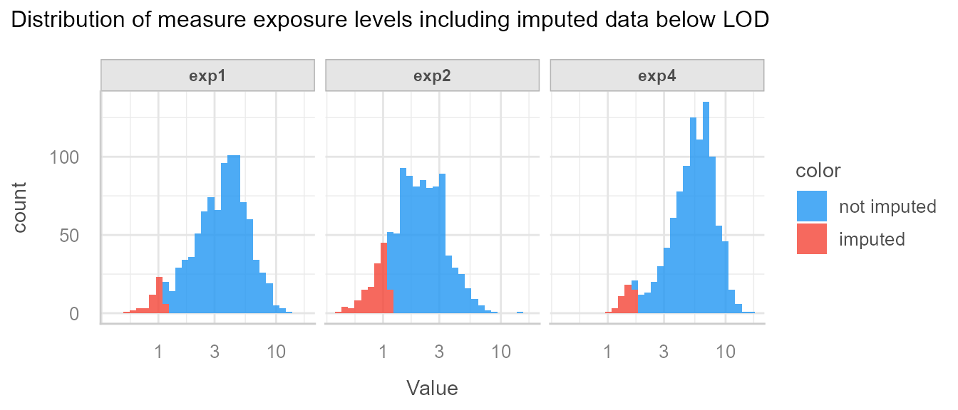
We see that imputed data is below LOD, and seem to have been drawn from the correct distribution.

Step 2: Standardise data on protocol variables

Next we want to standardise the filled-in values on protocol variables batch, prot1 and prot2, while taking into account the covariates season and cov1.

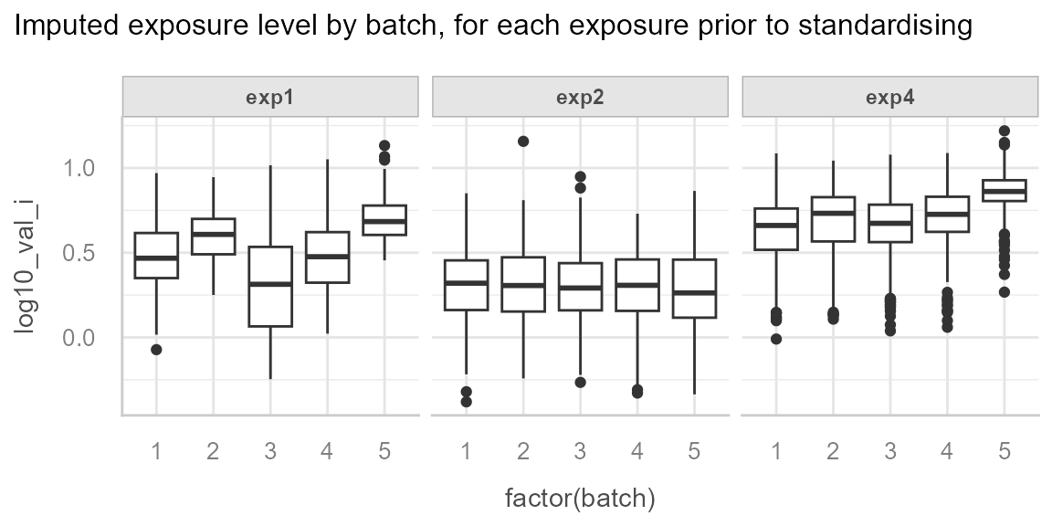
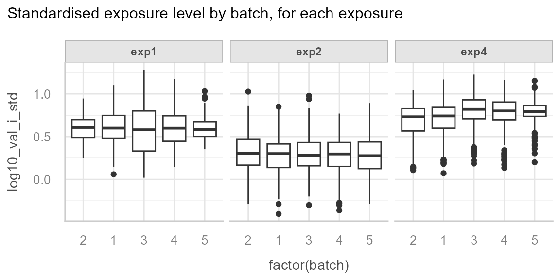
We start by describing the data.

We can observe the batch effect for exp1 and exp4:

And we can observe the effect of season for exp4:

ggplot(dt_imp, aes(x = factor(season), y = log10_val_i)) +
  geom_boxplot() +
  facet_wrap(~exp) +
  see::theme_lucid() +
  labs(
    title = "Imputed exposure level by season, for each exposure prior to standardising"
  )

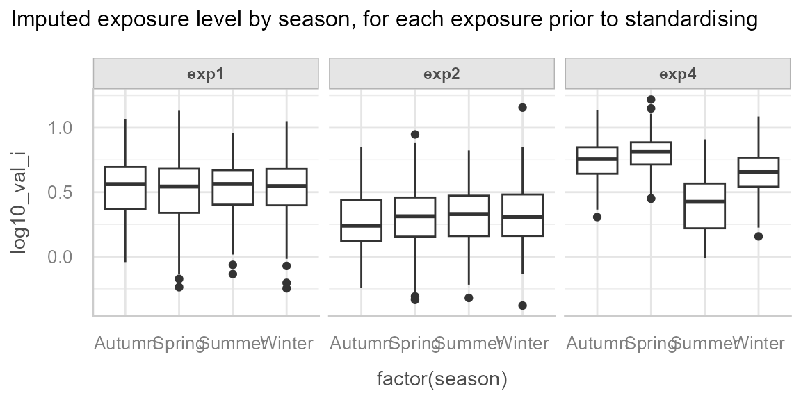
And finally we observe an unequal distribution of season by batch:

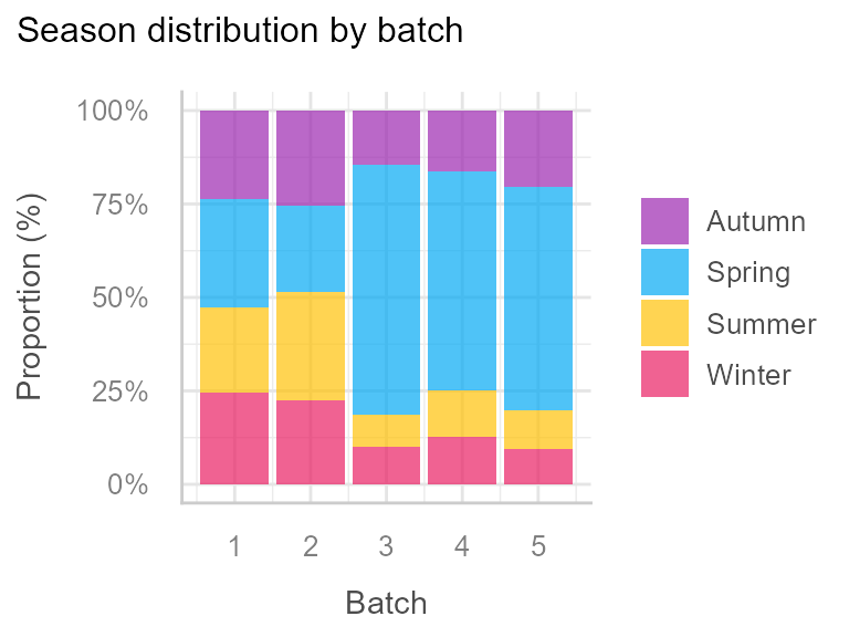
This justifies the inclusion of season as a covariate in the standardisation models, in order to differentiate the effect of batch from the effect of season, because we want to standardise for batch but not for season.

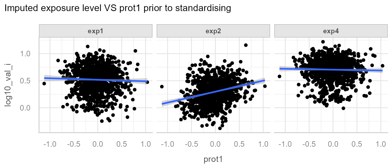
We can also observe the association between exp2 and prot1:

The goal of the standardisation process is to detect among all the protocol variables (batch, prot1 and prot2) which are associated with which exposure, and standardise each exposures for the specific protocol to which it is associated.

The first step of the standardisation process is to define potential protocol variables that might be associated with the variable to standardise and the extra covariates to be included in the model:

lst_prot_vars <- c("batch", "prot1", "prot2") 
lst_cov <- c("season", "cov1")

Then define which are the reference values for the categorical variables (e.g. if the reference value for batch is batch 2, all batches will be “aligned” with batch 2):

# set categorical variable reference values for categorical data
dt_imp <- dt_imp |>
  mutate(
    batch = relevel(factor(batch), ref = "2"),
    season = relevel(factor(season), ref = "Spring")
  )

Reference value for continuous protocol variables is the median [@mortamais_correcting_2012].

Once the protocol variables and the covariates have been listed and the reference values have been set, we can apply the standardisation function:

# Standardise 
dt_std <- dt_imp |>
  mutate(
    log10_val_i_std = standardise(
      var_to_std = "log10_val_i",               # variable to be standardised
      protocol_vars = lst_prot_vars,            # list of candidate protocol variables
      covariates = lst_cov,                     # optional list of covariates, defaults to NULL
      folder = "standardisation_outputs"        # folder where outputs are saved
    ),
    .by = exp                                   # grouping variable
  )

It is crucial to look at the standardisation process outputs and the data posterior to the standardisation step to make sure what was done matches what was expected.

All outputs are saved in the folder defined in the path argument.

If you want to inspect model diagnostics (linearity, residuals, homoscedasticity, etc.), you can enable the optional argument export_check_model = TRUE in the standardise() function. This will save model diagnostic plots produced by performance::check_model() in the same folder as the other outputs. This can help verify that linear model assumptions hold for the correction models.

We can first have a look at the associated protocol variables, that were used for the correction:

protocol_vars	exp1	exp2	exp4
batch	<2e-16	0.42	<2e-16
prot1	0.59	6.3e-16	0.91
prot2	0.58	0.78	0.55

We see that the correct variables were detected.

We can see the correction for the batch effect of exp1 and exp4:

We can note that there is still residual variability between batches for exp4, in our case this can be explained by the season effect for which we have not adjusted.

And the correction of exp2 for prot1:

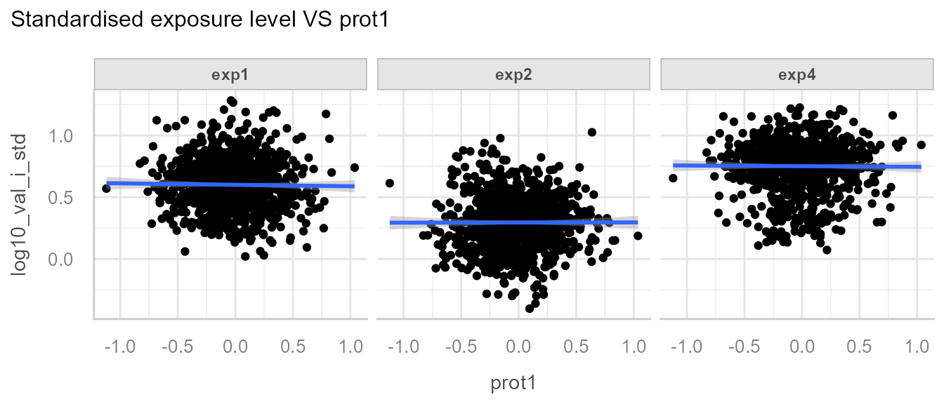
Note: The correction may not be so apparent, as realistic data likely possesses greater residual variability.